
Transformers?
Transformer is the underlying big idea behind unbelievable language models like ChatGPT, and GPT-4 which crate headlines all over the world these days. The Transformer is nothing but a deep neural network architecture introduced in 2017 by Vaswani et.al in their paper titled Attention is All You Need. In 2012 AlexNet brought hype to Computer Vision by bringing CNNs into the picture, and similarly, Transformers brought that hype to Language Processing in 2017. Transformer architecture was introduced as an alternative to the traditional Recurrent Neural network-based architectures like LSTM and GRU overcoming most of their drawbacks. The introduction of Transformers extended the boundaries of many branches of AI, even though it originated from a Natural Language Processing (NLP) paradigm. Thanks to those incredible ideas today we are witnessing accelerated progress toward Artificial General Intelligence (AGI), which was just a fairytale a few decades ago. In this post, I will try to explain the idea behind the Transformer architecture and you will realize why it works so well at the end.
Word Embeddings
Before moving into Transformers we should get the background cleared. Let us recall the idea of word embeddings first.
Computers cannot understand words or images as we perceive them. Computers need a numeric representation to understand anything. For images and videos, we use pixel-based representation (You can check my previous post about Digital Image Processing). The corresponding representation for words is word embeddings.
We can give a vector representation to words using different techniques. In the early days, statistical-based representations were used. Count vectorization, One-hot-encoding, and TF-IDF are some popular such methods. With the introduction of Word2Vec, the real idea of word embeddings came into play. That is the automated generation of vector representations for words rather than using hand-crafted features. This gave impressive results in those days when those embeddings not only gave vector representation for words but could embed the analogical meanings as well into the embeddings. As an example, using Word2Vec word embeddings we can verify the following word analogy is true.
King - Man + Woman ≃ Queen
How impressive that is! You can check this implementation by Tensorflow and see how impressive these word embedding representations are. Embeddings of similar words lie closer in the embedding space. GloVE and FastText also are global (fixed) word embedding representations similar to Word2Vec.
But there's a problem with these embeddings. They are fixed embeddings! So what's wrong with that? Check out the following example.
I got cold during the vacation due to that cold weather
Here the word cold in the two places has two meanings. The first one represents the disease and the second one represents the low-temperature condition. Therefore it is not that good to have the same embedding representation for the cold on these two occasions. That's where the idea of contextual word embeddings comes into the picture. That is the embeddings of words are not fixed. They depend on the context. The context in the sense, the neighbor words, and the meaning the words try to convey. The transformer architecture can generate really good contextual word embeddings using Attention mechanisms and that's where the real power of this architecture lies.
Self Attention
The idea behind self-attention is to give more contextual meaning to existing word embeddings. The words in a sentence (or phrase or document - whatever the linguistic unit we consider as the input) will pay attention to themselves and get more contextual meaning.
 |
Figure 1: High-Level Idea of Self-Attention |
Notion of Attention
Let's say we have a noisy time-series number sequence X1, X2, ... Xn and we want to have a filtered (noise eliminated) version of those numbers. From simple statistics, we know that taking the average will reduce random noise. Therefore a simple way is to take a weighted average to have a better version of our time-series data. Say we want to have a filtered version of the datapoint Xi. What we can do is, get a weighted average of the data points around Xi and take that value as an estimation for noiseless Xi. In this particular scenario, we can choose the weights in such a way that more weight will be given to the current data point and gradually reduce the weight for distant data points.
See Figure 2. The noisy data points (blue) should be filtered to get closer to the regression line (purple). We are doing a weighted average to achieve that. We have shown how the weights should be for two sample data points (datapoint at 6 - red and 8 - orange). The weights of the red datapoint are shown in the red curve and the orange is in the yellow curve. Assume that the weights are normalized (i.e. the sum of all the weights is one). This makes sense because more weight (attention) should be paid to the nearby data points. The weighting scheme here is based on proximity. The closer the data point is, the higher the assigned weight factor should be.
 |
| Figure 2: Weighted Average to Reduce Noise |
Dot Product
The dot product (a special case of inner product in Mathematics) between two vectors a and b is denoted by a.b, which is simply the sum of the elementwise products of the two vectors as shown in Equation 1.
 |
Equation 1: Dot Product Formula 1 |
This also can be represented as the product between the norms (i.e. magnitudes) of the two vectors multiplied by the cosine of the angle between the two vectors. See the Equation 2.
 |
Equation 2: Dot Product Formula 2 |
When the two vectors are unit vectors (i.e. ||a|| = ||b|| = 1), the dot product becomes the cosine of the angle between, which is called the cosine similarity (1 - cosine similarity = cosine distance) between the two vectors. Cosine similarity is a well-known similarity measurement among vectors. The more similar the two vectors are, the lesser the angle between them, and that means the larger the cosine similarity is.
Scaled Dot Product Attention
In transformer architecture, they have exploited the idea behind the dot product in order to add more contextual information to the embeddings. Figure 3 shows how we can simply improve an existing word embedding Xi, and have an added contextual information version of that Yi, using its neighboring word embeddings.
Recall how we reduced the noise in the time-series number sequence in Figure 2 by taking a weighted average, where the weight factors indicated how much attention we should provide to each of the data points in the sequence.
Now we will move on to our scenario. We can follow a similar approach here as well. We can add more context to a given word embedding by taking a weighted average of all the word embeddings in the input sentence but, we have a problem. The weighing mechanism cannot be proximity based since linguistic relationships are not based on proximity but based on the syntax (grammar) and semantics (meanings) of the language.
 |
Figure 3: Build a Contextually Rich Word Embedding |
As we discussed earlier, word embeddings already have the basic notion of linguistic information (can perform analogical arithmetic). Therefore we can use the word embeddings to find out the weighting factors.
First, we need to tokenize the input sentence (i.e. break it into tokens/words) and then take the word embeddings of all the words (the ideal term would be tokens but I am continuing with words). Now, we have some sort of high-level word embeddings for the words of a sentence (X1 .. Xn). Think that we want to include more contextual information to a particular word embedding among them, let's say to Xi.
As the first step, we take the dot product between Xi and all the other word embeddings in the sentence. Now we know that the dot product gives us some sort of similarity measure among vectors. The resultant vector is then normalized in order to form a unit vector (W1 ... Wn). This acts as our new weighting factors related to Xi which will represent how much Xi is related (attended) to each of the embeddings. Now, we can get the weighted sum of the initial word embeddings to get Yi, the new representation of Xi. This is the part you need to realize. Think and realize why Yi becomes a contextually-rich representation of Xi.
We can interpret this operation from a database search query point of view as well. Assuming a simple key-value database, a user query is served by returning the corresponding values of the keys that match with the user query. In the database case, we need exact matches to return values. In contrast, in the transformer case, it is not an exact match but rather a fuzzy match.
The above mechanism is static (i.e. no trainable parameters in it) and therefore we can not let a machine-learning approach extract any hidden relationships among the embeddings. We can add some trainable parameters to the process so that the above mechanism will become more robust. We can add trainable matrices Mk, Mq, and Mv as shown in Figure 4.
 |
| Figure 4: Include Trainable Matrices to the Attention Mechanism |
We can redraw the process in Figure 4 as per Figure 5. The trainable metrics Mk, Mq, and Mv can be represented by Linear layers with no bias terms (WX + b without b). All the dot product results can be found at once by arranging the vectors as metrics and then performing matrix multiplication (Matmul). Try to realize that Figure 4 and Figure 5 show the same arrangement in two different views.
By introducing the trainable parameters (weights of the Linear layers), now we can let the network learn new dot product-like attention mechanisms. Now we are not restricting but encouraging the network to freely learn complex relationships.
 |
Figure 5: A Different View of Figure 4 |
This mechanism of enriching the contextual representation of word embeddings is called the Scaled Dot product Attention. Figure 6 shows the diagram of this attention mechanism from the original paper. See that it is the same as we just discussed above. The formula for this is given in Equation 3.
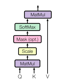 |
Figure 6: Scaled Dot Product Attention from the Paper |
 |
Equation 3: Scaled Dot Product Attention Formula |
Note that SoftMax does the normalizing. By default, none of the Q, K, and V metrics contain normalized vectors, and therefore dot products can grow large in magnitude, pushing the softmax function into regions where it has extremely small gradients (vanishing gradient problem). To counteract this effect, the dot products are scaled by 1/√dk where dk is the dimension of the keys matrix, therefore, the name Scaled Dot Product Attention.
Multi Head Attention
In a single sentence (input) we may need to learn multiple attention (relationship) mechanisms. In contrast to convolution neural networks (CNNs), there we stack multiple kernels to form a single filter, where every single kernel will learn to extract different image features (see my previous post for more details). In the same way, we can have multiple parallel Keys, Queries, and Values layers so that each layer (attention head) will learn different types of attention mechanisms (different types of contextual relationships among words) in the training process. If we add such parallel layers, Figure 5 can be extended to Figure 7.
 |
| Figure 7: Multi-Head Attention Version of Figure 4 |
The main difference here is, due to having multiple attention mechanisms we get multiple output vector representations for a given input vector (in CNN context similarly we get multiple channels in the output). Therefore those multiple outputs are concatenated (and sent through another linear layer) to form the final contextually-rich vector representation of the input. The authors have used Figure 8 in the paper to represent multi-head attention.
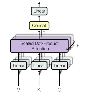 |
Figure 8: Multi-Head Attention from the Paper |
The formula associated with multi-head attention is given in Equation 4.
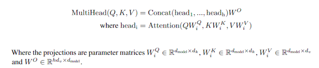
Equation 4: Multi-Head Attention Formula
What's Next
My Idea in this post was not to explain the entire Attention is All You Need paper but to give you an intuition of why this architecture works. If you got the ideas so far then you can go ahead and read the paper. There are many more cool ideas that I have not discussed here (Encoder-Decoder Attention, Masked Decoder Attention, Positional Encoding, Layer Normalization). All these ideas together make this architecture so powerful.
If you want further explanations check this blog post which is quite a popular post among the community. Some of the examples I used here were inspired by this video tutorial by Rasa. See you with a new post!
Comments
Post a Comment