ML Algorithms: Linear Regression

When, why, and how the business analyst should use linear regression - ufert.se | Eric Seufert

Introduction

This will be the first post of the series of posts on Machine Learning (ML) algorithms. I will be providing sample Python scripts to demonstrate the theories discussed in the posts. You can access all the code examples using this link.

Linear Regression is the first ML algorithm that any ML newcomer will learn in his study of ML algorithms. Linear Regression is a Supervised Learning algorithm as we mentioned in our previous post on What is Machine Learning?. It’s used to predict values within a continuous range (e.g. Prices, Sales, etc.) which means this method is used to solve regression problems (not classification problems) as we discussed in our previous post.

In other words, we can estimate a linear relationship between some input/ independent variables (features as we discussed in the previous post) and an output/ dependent variable using this method. The general relationship will look like this.

Equation 1: Linear Regression equation

Here

X1, X2, ... , Xm are the input/ independent variables,
f or Y is the output/ dependent variable and
b is called the bias term.
W1, W2, ... ,Wm are called the weight terms.

This may be more familiar for you with a single input. In that case, this relationship is reduced to,

Equation 2: Simple Linear Regression equation

which is nothing but the formula of a straight line.

In linear regression problems what we do is, using the data set (inputs and labels as we discussed in our previous post) we will find out the values of the weight terms (i.e. W1, W2, ..., Wn) and the bias term (i.e. b). This is the same as the Regression Analysis in Mathematics but the workflow may be different.

Math behind

Simple Linear Regression

Firstly I will prove the concept considering the single input case.

Let us assume the linear relationship between the input/ feature (x) and the output/ target variable is given by,

Equation 3: Simple Linear Regression equation

Here m is the weight and b is the bias.

In our data set we are given a set of (Xi, Yi) data points (i.e. {(X1, Y1), (X2, Y2), ..., (XN, YN)}). Assume the data set contains N number of data points. Our mission is to find out m and b such that the y=mx+b will give the best matching line for our data points.

In the following figure, the blue dots are our (Xi, Yi) data points, and finding the black line is our target.

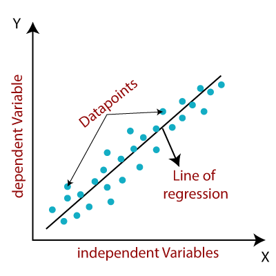Regression in Machine Learning - IBM Z and LinuxONE Community

Figure 1: Simple Linear Regression Graphically

Step 1: Initialize the variables

Initialize m and b with some arbitrary values. Now we have an equation for the regression line which is

Equation 4: Simple Linear Regression equation

Step 2: Calculate the predictions

Substitute our Xi values from the data set (i.e. {(X1, Y1), (X2, Y2), ..., (XN, YN)} to the above and get the results or the predictions (i.e. f(Xi) = mXi + b values). The error will be the difference between the Yi's and the f(Xi)'s.

Expression 1: Simple Linear Regression Error term

Step 3: Define the Cost Function

Take the Mean Squared Error of the step 2 results/ predictions (i.e. f(Xi)) and our actual target values (i.e. Yi). This is nothing but the mean of the squares of the error terms.

Equation 5: Simple Linear Regression Mean Squared Error

Here,

$N$ is the total number of observations (data points)
$\frac{1}{N} \sum_{i = 1}^{n}$ is the mean
$y_{i}$ is the actual value of an observation and $m x_{i} + b$ is our prediction for the current m and b

If we are to find the best fitting line, then we need to find m and b such that this MSE will be minimum.

We have to minimize the MSE with respect to m and b. So we have to consider the MSE expression as a function of m and b.

Equation 6: Simple Linear Regression cost function

Step 4: Calculate the gradients/ derivatives w.r.t. the variables

Now we need to find the partial derivatives of f(m, b) with respect to m and b. By differentiating the above expression we get,

Equation 7: Simple Linear Regression Gradient calculation

Note: Gradient Descent

Gradient descent is an optimization algorithm used to minimize some function by iteratively (again and again) moving in the direction of the steepest descent which can be found by the negative direction of the gradient.

When a ball is placed in a curvy area, it automatically rolls toward a valley. This is the notion behind this technique.

Consider the 3-dimensional graph below in the context of a cost function. We aim to move from the mountain in the top right corner (high cost) to the dark blue sea in the bottom left (low cost). The arrows represent the direction of the steepest descent (negative gradient/ derivative) from any given point–the direction that decreases the cost function as quickly as possible.

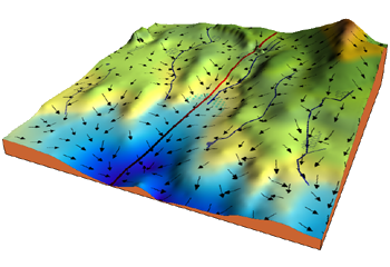Figure 2: A 3D cost function and maximum negative gradient (steepest descent) directions

The variables (weights and bias terms - m and b) are updated using the following formula. What this formula does is always move the new value of the variable towards a minimum value.

Equation 8: Gradient Descent - Weights and Bias Update Equation

Here J is the cost function and k is called the learning rate which determines how quickly you need to go towards the minimum. The learning rate should not be too large (weights may not get converged) or too small (will take more time to converge). If you need to learn more about Gradient Descent refer this article.

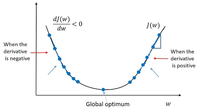003B Gradient Descent | Master Data Science

Figure 3: Gradient Descent - Single-variable Cost function minimization

Figure 4: Gradient Descent - Two-variable Cost function minimization
source: https://miro.medium.com/max/563/0*YfUeOTUhFHtLXyrI.gif

Step 5: Apply Gradient Descent to minimize the cost function

Now we know how to optimize a given cost function using the Gradient Descent method. We will iteratively update our m and b variables using the following Gradient Descent formulas until we reach the desired accuracy.

Equation 9: Simple Linear Regression weight and bias update equation

After reaching the desired accuracy, we have the final answers for m and b. That means we have found the best-fitting line for our data set.

N.B: Without using the Gradient Descent we could have solved this problem by finding the optimum values of the Cost function only by using the differentiation techniques. But this is the standard way to find optimum values of a cost function in Machine Learning. When it comes to problems with hundreds or thousands or even millions of trainable parameters, Gradient Descent comes in handy with Matrices.

The following flow chart shows the steps we discussed above in a compact manner.

Figure 5: Linear Regression Algorithm Flow chart

Multi-variable Linear Regression

Here the only difference is, we have multiple features/ inputs (Xi) that determine the output (Y) but the relationship is still linear.

Equation 10: Multiple Linear Regression Equation

There is one special thing you should do in multi-variable cases. That is you should do data normalization before doing the training.

Normalization

As the number of features grows, the ranges of different features can be different. As an example while one feature ranges between 0 and 1, another feature can range between 0 and 1000. So when it comes to estimating the relationship, some ML algorithms may not be good enough to equally treat both these features. Perhaps the algorithm may not get converged at the training phase. When we bring all the features to the same scale/ range this issue will not come anymore. The following figure clearly shows the impact of data normalization for a smooth convergence in the training process.

Figure 6: Gradient Descent without and with data normalization

Another issue is calculating gradients takes longer to compute when the numbers are very large. We can speed this up by normalizing our input data to ensure all values are within a common small range. There are different normalization techniques. A few popular ones can be listed as follows.

Z-score Normalization:

Subtract the mean and divide by the standard deviation.

Equation 11: Z-score relationship

Min-Max normalization:

Subtract the minimum value and divide it by the range (max minus min).

normalization using the min-max function

Equation 12: MinMax normalization relationship

Logistic Normalization:

Apply the logistic function.

formula for normalization by logistic function

Equation 13: Logistic function

Normalization is especially important for datasets with high standard deviations or differences in the ranges of the attributes.

Training Process

The error will be the same as before but the expression is a bit lengthy.

Expression 2: Multiple Linear Regression Error term

The cost function( here MSE - mean of the squares of errors) will be improved as follows. (Note that m number of features and n number of data points)

Equation 14: Multiple Linear Regression Mean Squared Error

The Gradients with respect to the weights and the bias can be found same as before.

Equation 15: Multiple Linear Regression Gradient Calculation

Usage of Matrices

But if you use matrices you can calculate all the gradients at once rather than writing separate lines of code to calculate the gradients for each weight term.

The relationship between features and the target variable can be written as Y = XW + b which will have the following meaning.

Equation 16: Multiple Linear Regression Matrix form 1

The error can be calculated in matrices as follows.

Equation 17: Multiple Linear Regression Error in Matrix Form

And the gradients can be found using the following matrix relationship (check with Equation 15 whether the same thing happens here as well). You have to calculate the gradient with respect to the bias term separately in this form. But there is another way in which we can find all the gradients in a single line.

Equation 18: Multiple Linear Regression Gradient calculations in Matrix form

If you can define the X matrix in the following form, you can merge both weights and bias terms into a single matrix so that you can calculate all the gradients at once using Equation 18. The relationship will be simplified to Y = XW

Equation 19: Multiple Linear Regression Matrix form 2

Code Examples

Some Python code examples to demonstrate what we have discussed so far have been uploaded to this location. You can download them and see how these theories can be applied to solve some real-world problems.

For more posts visit: https://iamkasunimesha.blogspot.com/
Code repository: https://github.com/Kasun-Imesha/Explore-science-and-Mathematics

simple_regression.py - pure python implementation of simple linear regression
simple_regression_numpy.py - simple linear regression implemented using numpy library
multivariable_regression_matrix.py - multi-variable regression implementation with weight and bias updates separately
multivariable_regression_matrix_type2.py - multi-variable regression implementation with a single matrix for weights and bias as discussed at the end of the previous chapter.
multivariable_regression_matrix_numpy.py - numpy implementation of the previous script

Note:

In all the code examples given in the above link, the algorithms have been implemented from scratch. Some of those implementations may be slower (pure implementations are slower than numpy implementations). There are libraries where all those Machine Learning algorithms have been implemented in optimized ways. Scikit-learn is such a Python library where most of the traditional ML algorithms have been implemented in optimized ways. You just need a few lines of code to find regression coefficients but to learn the basics you have to go from scratch.

Explore Science and Mathematics

Search This Blog